Getting started
The INDRA API requires an API Access Key to be provided in the header for each API request made. To request an API Access Key, please email the API team at indra@csiro.au and include the following information:
- full name
- organisation
- purpose for using the API
- intended audience (e.g. personal, customers).
The API service is currently available for free during an evaluation period. The API service continues to be developed and is therefore subject to changes.
Your Access Key will be a 32-character string containing random letters and numbers. The X-API-Key header should then be set to this value. For example, if using curl to make the API request, you would add the parameter:
-H 'X-API-Key: YOUR_ACCESS_KEY'
The Swagger interface for the API can be accessed at: dev.indraweb.io.
This provides brief documentation for each endpoint available as well as an interactive interface to try out
various endpoints and parameter options. To enable the interactive endpoints, you first need to Authorize by
entering your API Access Key in the popup box. First, click on the
 button on the right side of the screen and you'll be presented with a popup window where you can enter your
key.
button on the right side of the screen and you'll be presented with a popup window where you can enter your
key.
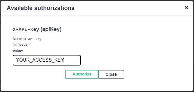
Enter your API Access Key in the Value box and click on the Authorize button, then the Close button to close
the popup window (do not logout here!). You should now see that the padlock icons for each endpoint are
closed.

All of the endpoints are simple GET requests and are grouped by functionality. To try out a particular
endpoint, click on it to expand its documentation and input parameter form. You must then click on the
 button to enable all of the input parameter
boxes/dropdowns. Default values have been provided for each parameter, so all you need to do to run it is
click on the Execute button below the input parameters. The example GET request, including a curl example,
with parameter values set is then shown below, along with the full JSON response.
button to enable all of the input parameter
boxes/dropdowns. Default values have been provided for each parameter, so all you need to do to run it is
click on the Execute button below the input parameters. The example GET request, including a curl example,
with parameter values set is then shown below, along with the full JSON response.
If an invalid input parameter is provided or a required parameter is missing, the JSON response will contain an error message describing the problem. For example, if the startYear parameter is set to 1920, the following response will be returned:
{ "errorMessages": [ "Invalid start and/or end year, valid year range is 1961 to 2024" ] }
About the data
The INDRA API utilises the following data for delivery at national scale:
- Temperature and rainfall observation data from the Bureau of Meteorology.
- Relative humidity and solar radiation observation data from the European Centre for Medium-Range Weather Forecasts, using its ERA5 reanalysis dataset.
- Projected future rainfall, temperature, relative humidity and solar radiation data from Climate Change in Australia, using its Application-Ready dataset.
- Observed and projected future soil moisture and potential evapotranspiration data from the Bureau of Meteorology.
- Historical Forest Fire Danger Index (FFDI) data is calculated using the Bureau of Meteorology's AGCD for precipitation and temperature, and NCEP-NCAR for wind speed.
- FFDI projection data is calculated using the Climate Change in Australia's ESCI project datasets. These were bias corrected using QME bias correction (see https://doi.org/10.1071/ES20001). The FFDI data obtained is also bias corrected in post processing using QME. More information on this is available in ESCI Technical Report: Downscaling and evaluating datasets and Extreme temperature, wind and bushfire weather projections using a standardised method.
- Past average monthly wind speeds are derived from the CSIRO's Near-Surface Wind Speed dataset.
- Elevation data from the Australian National University's Digital elevation model dataset.
These datasets are all provided as ‘gridded’ datasets and are produced by combining data from the Bureau of Meteorology's weather stations around Australia and presenting it on a uniform national 5x5 km grid using a technique called ‘interpolation’. Interpolation allows us to ‘fill in the gaps’ between the weather stations. This technique takes account of topography and aims to give a confident estimate of rainfall/temperature including in areas with high topography. The Bureau has a vast network of weather stations across Australia. Weather stations provide reliable data at point locations. However, it's not possible to place weather station equipment every few kilometres across the expanse of Australia. The gridded data allows us to provide a reliable estimate of conditions in data-sparse areas consistently. This means that the closest grid(s) to you will represent data from several nearby weather stations. For this reason, the data at your grid point might not be the same as that from any single gauge.
For temperature, precipitation, relative humidity and solar radiation, eight climate models: ACCESS1-0, CESM1-CAM5, CNRM-CM5, CanESM2, GFDL-ESM2M, HadGEM2-CC, MIROC5 and NorESM1-M (see Climate Change in Australia for details) were selected to be representative of the range of seasonal temperatures and rainfall across Australia.
The soil moisture and potential evapotranspiration data is sources from the Australian Water Outlook's National Hydrological Projections. This consists of 16 ensemble models, labelled ens00 to ens15.
The 16 Forest Fire Danger Index (FFDI) projection models and ensembles included are detailed in the following table:
| Model family | Source GCM name | Ensemble |
|---|---|---|
| CCAM | ACCESS1-0, CanESM2, GFDL-ESM2M, MIROC5, NorESM1-M | |
| BARPA | ACCESS1-0 | |
| NARCliM 1.5 | ACCESS1-0, ACCESS1-3, CanESM2 | NARCLIMj |
| NARCliM 1.5 | ACCESS1-0, ACCESS1-3, CanESM2 | NARCLIMk |
| GCM | ACCESS1-0, CNRM-CM5, GFDL-ESM2M, MIROC5 |
There is no single "best" model and climate projections differ between models. As such, API users are strongly advised to include output from all available models in their analyses rather than using results from a single climate model. In addition, API users are encouraged to include analyses for both emissions scenarios (RCP4.5, RCP8.5) to incorporate a range in future climates due to different possible global emission pathways.
For each future projection period there are approximately 30 years of data. All these years are used to calculate the climatology centred on the selected projection period (e.g. 2050). Users are recommended to evaluate statistics across all these years. Selecting a single or a few years for analyses will not represent the projected time period appropriately.
All /projections endpoints will return data for all climate models available. It is up to the API client software to calculate the multi-model-mean or other statistics from this data, noting that we strongly advise using data from all the climate models and not an individual one.
When an API request is received, the input coordinates are first converted into a corresponding grid cell reference for the underlying data source. All grid cell dimensions are 0.05 x 0.05 degrees. Therefore, requests with coordinates that fall within the same grid cell will always return the same response, even if they are a few kms apart.
The temperature, precipitation, humidity and solar radiation data has the following geographical extent: 111.975, -44.525 to 156.275, -9.975 (grid dimensions 886 x 691)
The soil moisture and potential evapotranspiration data uses an alternative grid: 111.975, -44.025 to 154.025, -9.975 (grid dimensions 841 x 681)
The API will return an error message if the input coordinates don't fall within a grid cell. For example:
{ "errorMessages": [ "Invalid coordinates, must be within 111.975,-44.525 and 156.275,-9.975" ] }
While some observation data is available for all grid cells (e.g. temperature), most datasets cover land areas only and will return an empty response if you provide coordinates that are well out into the ocean. For example, the request
/projections?lon=113.1289&lat=-35.2819&variable=precip&frequency=monthly&years=2016-2045&emission=rcp45
will return the following empty response:
{ "data": [] }
Endpoint options
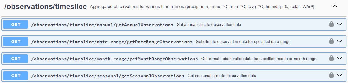
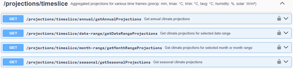
There are two main types of endpoints: /observations and /projections. The /observations endpoints always retrieve historical observation data, whereas the /projections endpoints retrieve climate projections data from many different climate models. For every /observations endpoint there is usually a /projections equivalent. Some exceptions to this are due to the availability/storage requirements of daily projection data and so the /date-range endpoint, which uses daily data, may not be present at this time.
The following shows the /observations and /projections timeslice endpoints, where you can see the matching endpoints for each time frame option available.
Note: Including the /getXYZ operation name at the end of each endpoint, as listed in the Swagger interface, is not necessary. Many of the example requests below have excluded this for readability purposes.
Some endpoints can be used to retrieve the original data for the specified location, as daily (observations only) or monthly values. All other endpoints perform some sort of aggregation/computation to provide to provide a yearly value for the specified variable. The original data endpoints are:
/observations/getObservations
/observations/soil-moisture/getSoilMoisture
-
/observations/evapotranspiration/getEvapotranspiration
-
/observations/ffdi/getFFDI
-
/observations/spi/getSPII
/projections/getProjections
-
/projections/soil-moisture/getSoilMoistureProjections
-
/projections/evapotranspiration/getEvapotranspirationProjections
-
/projections/spi/getSPIProjections
-
/projections/spi/getSPIProjections
There are usually four ways of specifying a specific yearly time frame and these are provided as different endpoints for each endpoint group: /annual, /seasonal, /month-range and /date-range.
Annual
The /annual endpoints will always return aggregate data for a calendar year (1 January to 31 December), with one value per year. For example, the request
/observations/timeslice/annual?lon=149.1289&lat=-35.2819&variable=precip&startYear=1961&endYear=2023
will return the total annual precipitation received for each year from 1961 to 2023 at the specified location.
Seasonal
The /seasonal endpoints have a season input parameter which can be one of summer, autumn, winter, or spring. Note that summer values will be assigned to the year in which summer starts, e.g. summer 2020 is Dec 2020 to Feb 2021.
Month range
The /month-range endpoints have a monthRange input parameter which can be set to either a specific month or consecutive month range. If specifying a single month, then the month name can either be the abbreviated three-character version or the whole month name, e.g. apr or october. If specifying a consecutive, then the month range is specified using the first letter of each month in the sequence. e.g. mjjaso represents the months from May to October inclusive. Month ranges can cross a year-end, e.g. djf, but cannot be longer than 12 months. If the month range spans a year-end then the year assigned to the result will be the year in which the month range starts. e.g. ondjfm 2020 is Oct 2020 to Mar 2021.
Date range
The /date-range endpoints have startDate and endDate input parameters, which need to be specified in MM-DD format. For example, 07-10 for the 10th of July. To specify a date range that spans a year-end, the endDate will be earlier than the startDate, e.g. startDate=12-01&endDate=05-15, represents the date range from 1st December to 15th May. The date range must be at least 28 days in length.
Many of the endpoints have a variable as an input parameter. The following describes the various variable options, noting that sometimes only a subset of these is available.
precip
Precipitation, presented in millimetres (mm), is most often rain, but also includes other forms such as snow. Observations of daily rainfall are nominally made at 9 am local clock time and record the total precipitation for the preceding 24 hours. Endpoints with variable=precip that return a mm value, calculate the total precipitation recorded for the specified time frame. For example, the request
/observations/timeslice/seasonal?lon=149.1289&lat=-35.2819&variable=precip&season=winter&startYear=1961&endYear=2022
returns the total winter precipitation received each year at that location.
tmin and tmax
Air temperature, presented in degrees Celcius (°C), is measured in a shaded enclosure at a height of approximately 1.2 m above the ground. Maximum and minimum temperatures for the previous 24 hours are nominally recorded at 9 am local clock time. The minimum temperature is recorded against the day of observation, and the maximum temperature against the previous day. Endpoints with variable=tmin or tmax calculate the average daily minimum or maximum temperature over the specified time frame. For example,
/observations/timeslice/month-range?lon=149.1289&lat=-35.2819&variable=tmin&monthRange=july&startYear=1961&endYear=2022
returns the average daily minimum temperature observed in the month of July each year.
tavg
Measured in °C, is the average daily temperature and is calculated as the average of the minimum and maximum daily temperatures. This variable is only available on some endpoints.
humidity
Relative humidity at 2 metres, measured as a % number from 0 to 100.
solar
Average daily downward shortwave radiation at the Earth's surface, measured in W/m².
RCP4.5 is a medium emissions scenario where greenhouse gas emissions peak around 2040, and then decline to
below current emission levels by 2100.
RCP8.5 is a high emissions scenario and describes a future with greenhouse gas emissions continuing to
increase to 2100.
All /projections endpoints have an emissions input parameter which can be either 'rcp45', 'rcp85' or 'rcp45,rcp85' to retrieve data for both scenarios together.
The /threshold endpoints have constraints placed on the specified threshold values which are dependant on the variable input. A 400 error response will be returned if the value specified is outside the range. These constraints are as follows:
| Variable(s) | Minimum | Maximum |
|---|---|---|
| precip | 0 | 20 |
| tmin, tmax, tavg | -20 | 50 |
| humidity | 0 | 100 |
| solar | 0 | 350 |
The threshold operator input parameters usually need to be URL-encoded. A list of operators and their URL-encoded equivalent is shown below.
| Operator | Meaning | URL-encoded |
|---|---|---|
| <= | less than or equal to | %3C%3D |
| < | less than | %3C |
| > | greater than | %3E |
| >= | greater than or equal to | %3E%3D |
JSON responses
This response contains an array of 12 (for monthly) or 365/366 (for daily) values for each year from startYear to endYear inclusive. If the endYear is the current and therefore incomplete year, only the observed values to date will be returned. For example, the request
/observations?lon=149.1289&lat=-35.2819&variable=precip&frequency=monthly&startYear=2022&endYear=2024
(get monthly precipitation data from 2022 to 2024) returns the following JSON:
{
  "data" : [ {
    "year" : 2022,
    "values" : [ 102.9, 83.1, 29.4, 80.4, 103.6, 26.2, 17.9, 128.0, 75.6, 182.1, 100.8, 41.7 ]
  }, {
    "year" : 2023,
    "values" : [ 71.3, 50.1, 79.8, 81.6, 54.2, 41.1, 9.3, 23.2, 15.8, 32.7, 119.8, 92.5 ]
  }, {
    "year" : 2024,
    "values" : [ 124.9, 54.5, 28.9, 75.2 ]
  } ]
}
This response contains an array of year/value pairs, one for each year in the specified year range. For example, the request
/observations/threshold/annual?lon=149.1289&lat=-35.2819&variable=tmin&startYear=2021&endYear=2023&threshold=2&operator=%3C
which counts the number of days per year with a tmin < 2°C (note the URL encoded operator value '<'), returns the following JSON:
{
  "data": [
    {
      "year": 2021,
      "value": 89
    },
    {
      "year": 2022,
      "value": 66
    },
    {
      "year": 2023,
      "value": 85
    }
  ]
}
This response contains event summary data for the entire year range specified, this is used by endpoints that dealt with multi-year events such as droughts and pluvial flooding. For example, the request
/observations/spi/events/getSPIEventData?lon=149.1289&lat=-35.2819&startYear=1961&endYear=2023&eventType=wet,dry
which retrieves summary "wet" and "dry" event data for the year range from 1961 to 2023 inclusive, returns the following JSON:
{
  "data" : [ {
    "yearRange" : "1961-2023",
    "eventType" : "wet",
    "avgDuration" : 9.642858,
    "eventCount" : 14
  }, {
    "yearRange" : "1961-2023",
    "eventType" : "dry",
    "avgDuration" : 8.263158,
    "eventCount" : 19
  } ]
}
This response contains arrays of 12 monthly values for each year within the specified year range and RCP emissions scenario. For example, the request
/projections?lon=149.1289&lat=-35.2819&variable=tmax&frequency=monthly&years=2036-2065&emission=rcp45
retrieves the projected monthly maximum temperatures for the year range 2036-2065 and emission scenario RCP4.5. Data for all eight climate models is returned in the response. An extract of the full JSON response is shown here:
{
  "data" : [ {
    "yearRange" : "2036-2065",
    "model" : "ACCESS1-0",
    "rcp" : "rcp45",
    "yearValues" : [ {
      "year" : 2036,
      "values" : [ 31.9, 28.6, 26.3, 23.6, 17.0, 12.4, 12.1, 13.3, 20.8, 23.5, 23.5, 27.1 ]
    }, {
      "year" : 2037,
      "values" : [ 30.5, 31.3, 25.6, 21.8, 17.4, 13.4, 12.9, 18.7, 18.9, 23.9, 31.0, 29.0 ]
    }, {
      "year" : 2038,
      "values" : [ 29.9, 32.2, 28.4, 19.2, 16.6, 12.2, 12.4, 14.7, 18.5, 21.8, 22.9, 25.9 ]
    }, {
    ...
    }, {
      "year" : 2065,
      "values" : [ 32.0, 28.5, 26.1, 23.0, 17.9, 14.3, 14.0, 13.7, 18.9, 22.4, 25.1, 25.6 ]
    } ]
  }, {
    "yearRange" : "2036-2065",
    "model" : "CESM1-CAM5",
    "rcp" : "rcp45",
    "yearValues" : [ {
      "year" : 2036,
      "values" : [ 32.8, 28.7, 25.5, 24.0, 17.5, 12.9, 12.7, 13.5, 19.9, 22.3, 22.8, 28.1 ]
    }, {
      "year" : 2037,
      "values" : [ 31.4, 31.4, 24.9, 22.2, 17.9, 13.8, 13.5, 18.8, 18.0, 22.8, 30.3, 30.1 ]
    }, {
      "year" : 2038,
      "values" : [ 30.8, 32.3, 27.6, 19.6, 17.1, 12.7, 12.9, 14.9, 17.5, 20.6, 22.2, 26.9 ]
    }, {
    ...
    }, {
      "year" : 2065,
      "values" : [ 33.0, 28.6, 25.4, 23.4, 18.4, 14.8, 14.6, 13.9, 17.9, 21.3, 24.5, 26.6 ]
    } ]
  }, {
    "yearRange" : "2036-2065",
    "model" : "CNRM-CM5",
    "rcp" : "rcp45",
    "yearValues" : [ {
      "year" : 2036,
      "values" : [ 32.7, 28.5, 26.4, 22.8, 16.7, 12.2, 11.4, 13.4, 20.1, 22.5, 22.5, 28.0 ]
    }, {
      "year" : 2037,
      "values" : [ 31.3, 31.3, 25.8, 21.0, 17.1, 13.1, 12.2, 18.7, 18.2, 22.9, 30.0, 29.9 ]
    }, {
      "year" : 2038,
      "values" : [ 30.7, 32.2, 28.5, 18.4, 16.3, 12.0, 11.6, 14.8, 17.7, 20.8, 21.9, 26.7 ]
    }, {
   ...
}
Like the AggregateObservations JSON response, the AggregateProjections contains arrays of year/value pairs for each year range, climate model and RCP combination, as specified by the input parameters. For example, this request
/projections/threshold/annual?lon=149.1289&lat=-35.2819&variable=tmax&years=2056-2085&emission=rcp85&threshold=35&operator=%3E
(note the URL encoded operator parameter value '>') retrieves the projected number of days per year where the maximum temperature is greater than 35, for year range 2056-2085 and emissions scenario RCP8.5. An extract of the full JSON response is shown here:
{
  "data" : [ {
    "yearRange" : "2056-2085",
    "model" : "ACCESS1-0",
    "rcp" : "rcp85",
    "yearValue" : [ {
      "year" : 2056,
      "value" : 24.0
    }, {
      "year" : 2057,
      "value" : 43.0
    }, {
      "year" : 2058,
      "value" : 39.0
    }, {
    ...
    }, {
      "year" : 2085,
      "value" : 20.0
    } ]
  }, {
    "yearRange" : "2056-2085",
    "model" : "CESM1-CAM5",
    "rcp" : "rcp85",
    "yearValue" : [ {
      "year" : 2056,
      "value" : 24.0
    }, {
      "year" : 2057,
      "value" : 42.0
    }, {
      "year" : 2058,
      "value" : 37.0
    }, {
    ...
}
Like the YearRangeObservations JSON response, the YearRangeProjections contains event summary data each year range, climate model and RCP combination, as specified by the input parameters. For example, the request
/projections/spi/events/getProjectedSPIEventData?lon=149.1289&lat=-35.2819&years=2056-2085&emission=rcp85&eventType=dry,wet
retrieves summary "wet" and "dry" event data for year range 2056-2085 and emissions scenario RCP8.5. An extract of the full JSON response is shown here:
{
  "data" : [ {
    "yearRange" : "2056-2085",
    "model" : "ACCESS1-0",
    "rcp" : "rcp85",
    "eventType" : "dry",
    "avgDuration" : 8.0,
    "eventCount" : 7
  }, {
    "yearRange" : "2056-2085",
    "model" : "ACCESS1-0",
    "rcp" : "rcp85",
    "eventType" : "wet",
    "avgDuration" : 8.8,
    "eventCount" : 5
  }, {
    "yearRange" : "2056-2085",
    "model" : "CanESM2",
    "rcp" : "rcp85",
    "eventType" : "dry",
    "avgDuration" : 7.75,
    "eventCount" : 8
  }, {
    "yearRange" : "2056-2085",
    "model" : "CanESM2",
    "rcp" : "rcp85",
    "eventType" : "wet",
    "avgDuration" : 6.75,
    "eventCount" : 8
  }, {
   ...
}
Calculation details
The /soil-moisture endpoints behave in the same way as the others, with the soil moisture values expressed as percentage values from 0 to 1. To enable the conversion to mm, an additional soil capacity component is included in the JSON response. This provides the mm capacity of the soil at three different depths: upper, lower and deep. For example:
{
  data: [...],
  soilCapacity: {
    upper: 36.018295,
    lower: 206.18056,
    deep: 497.20667
  }
}
My Climate View uses the combined upper and lower values to convert the soil moisture percentages to mm values. i.e. soil moisture in mm = (soilCapacity.upper + soilCapacity.lower) x soil moisture percentage.
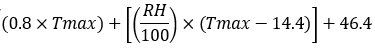
The /thi endpoints provide data that can indicate various levels of livestock heat stress. The THI calculations for each livestock type are calculated on the fly using the following formulas. The THI is calculated using daily data and the number of days where the THI exceeds the specified threshold is returned in the response. Suggested daily THI thresholds are listed in the tables below.
Beef

| Classification | Threshold |
|---|---|
| Mild heat stress for all breeds | 72–77 |
| Significant heat stress for Bos taurus | 78–86 |
| Significant heat stress for all breeds | 87–98 |
| Severe heat stress for all breeds | ≥ 99 |
THI equation reference: Wang, Xiaoshuai & Bjerg, Bjarne & Choi, Christopher & Zong, Chao & Zhang, Guoqiang. (2018). A review and quantitative assessment of cattle-related thermal indices. Journal of Thermal Biology. 77. https://doi.org/10.1016/j.jtherbio.2018.08.005
THI thresholds reference: Cowan, T., Wheeler, M.C., Cobon, D.H., Gaughan, J.B., Marshall, A.G., Sharples, W., McCulloch, J. and Jarvis, C., 2024. Observed Climatology and Variability of Cattle Heat Stress in Australia. Journal of Applied Meteorology and Climatology, 63(5): 645-663. https://doi.org/10.1175/JAMC-D-23-0082.1
Pork
| Classification | Threshold |
|---|---|
| Normal | < 75 |
| Moderate heat stress warning | ≥ 75 |
THI equation reference: Hahn, G.L., Gaughan, J.B., Mader, T.L. and Eigenberg, R.A., 2009. Thermal indices and their applications for livestock environments. In: J.A. DeShazer (Editor), Livestock energetics and thermal environment management. American Society of Agricultural and Biological Engineers, pp. 113-130. doi.org/10.13031/2013.28298
THI thresholds reference: NWSCR, 1976. Livestock Hot Weather Stress. In: N.W.S.C.R. (NWSCR) (Editor), Regional Operations Manual Letter C-31-76, Kansas City, MO, USA
Dairy
| Classification | Threshold |
|---|---|
| Unstressed | < 72 |
| Mild (in-calf rates can be reduced) | 72–74 |
| Moderate (in-calf rates and milk yield can be reduced) | 75–77 |
| High (in-calf rates and milk yield can be seriously affected) | 78–81 |
| Severe (in-calf rates can be reduced, very significant milk yield reduction and potentially death) | ≥ 82 |
THI equation reference: Nidumolu, U., Crimp, S., Gobbett, D., Laing, A., Howden, M., Little, S., 2014. Spatio-temporal modelling of heat stress and climate change implications for the Murray dairy region, Australia. International Journal of Biometeorology 58, 1095-1108. doi.org/10.1007/s00484-013-0703-6
THI thresholds reference: Dairy Australia, 2019. Cool Cows Booklet, Southbank, Victoria. nla.gov.au/nla.obj-2970730951
Sheep
| Classification | Threshold |
|---|---|
| No stress | < 22.2 |
| Moderate | ≥ 22.2 and < 23.3 |
| Severe | ≥ 23.3 and < 25.6 |
| Extreme | ≥ 25.6 |
THI thresholds reference: Marai, I.F.M., El-Darawany, A.A., Fadiel, A. and Abdel-Hafez, M.A.M., 2007. Physiological traits as affected by heat stress in sheep-A review. Small Ruminant Research, 71(1-3): 1-12. doi.org/10.1016/j.smallrumres.2006.10.003
GDD = 0
For each day within the specified date range:
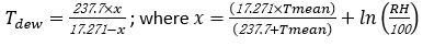
Tavg = (Tmax + Tmin) / 2
GDD += if (Tavg > baseTemp): Tavg - baseTemp; else 0
Different commodities will have different base temperatures, for wine grapes it is set to be 10 °C.
The /chill-portion endpoints provide chill accumulation data (measured in Chill Portions) which is calculated using the Dynamic Model. Due to the complex nature of the calculations, chill portion data has been pre-calculated for three different month ranges only. This differs from all the other endpoints which do their calculations on the fly. This is why there is only a single observations and projections endpoint for chill-portions, with the month range required specified as an input parameter.
References:
- Luedeling, E., Zhang, M., Luedeling, V., & Girvetz, E. H., 2009. Sensitivity of winter chill models for fruit and nut trees to climatic changes expected in California's Central Valley. Agriculture, Ecosystems & Environment, 133(1-2), 23-31. doi.org/10.1016/j.agee.2009.04.016.
- Darbyshire, R., Webb, L., Goodwin, I., & Barlow, S., 2011. Winter chilling trends for deciduous fruit trees in Australia. Agricultural and forest meteorology, 151(8), 1074-1085. doi.org/10.1016/j.agrformet.2011.03.010
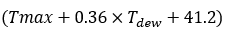
Cold exposure is defined as days with very high chill index during lambing season (date range is region specific). The chill index (Donnelly, 1984) estimates lamb cold exposure based on weather conditions and is used by the Bureau of Meteorology to issue ‘sheep grazier alerts’ (Cowan et al., 2022).
Cold exposure = number of days where Chill index > 1100
References:
- Cowan, T., Wheeler, M.C., de Burgh-Day, C., Nguyen, H. and Cobon, D., 2022. Multi-week prediction of livestock chill conditions associated with the northwest Queensland floods of February 2019. Scientific Reports, 12(1): 5907.10.1038/s41598-022-09666-z
- Donnelly, J.R., 1984. The productivity of breeding ewes grazing on lucerne or grass and clover pastures on the tablelands of Southern Australia. III. Lamb mortality and weaning percentage. Australian Journal of Agricultural Research, 35(5): 709-721.10.1071/AR9840709
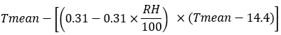
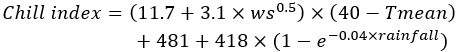
The /ffdi endpoints provide counts of days with a calculated FFDI that exceeds the specified danger threhold. The FFDI is based on combining daily maximum temperature (at a height of 2 m) with mid-afternoon values of relative humidity (at a height of 2 m) and wind speed (at a height of 10 m) as well as a drought factor representing fuel availability (based on rainfall and temperature to indicate a temporally accumulated fuel moisture deficit). See references below for full FFDI calculation details.
| Danger level | Threshold |
|---|---|
| Very high | 25 |
| Severe | 50 |
| Extreme | 75 |
References:
- The Bureau of Meteorology's Gridded Fire Weather Climatology Metadata.
- Dowdy, A.J., Ye, H., Pepler, A. et al. Future changes in extreme weather and pyroconvection risk factors for Australian wildfires. Sci Rep 9, 10073 (2019). https://doi.org/10.1038/s41598-019-46362-x
- Dowdy Andrew J. (2020) Seamless climate change projections and seasonal predictions for bushfires in Australia. Journal of Southern Hemisphere Earth Systems Science 70, 120-138. https://doi.org/10.1071/ES20001
The /spi endpoints provide Standardised Precipitation Index (SPI) (Mckee, Doesken, & Kliest, 1993) data, which is a meteorological index for characterizing drought and pluvial flooding events.
The SPI is simply a transformation of the cumulative distribution of precipitation time series data which follows a gamma distribution, into a standardized normal distribution. For fitting the gamma distribution, we used L-moments (Hosking, 1990) for initial guess and then used maximum likelihood estimation (MLE). For the maximum likelihood estimation, the Broyden-Fletcher-Goldfarb-Shanno (BFGS) algorithm was used.
The SPI has been developed to quantify drought and pluvial flooding events at multiple time scales. For example, 12 month values were used in (Kirono, Round, Heady, Chiew, & Osbrough, 2020), whereas 6 month values were used in (Martin, 2018) and values for 3, 6, 8, 12, 18 and 24 months were used in (Lloyd-Hughes & Saunders, 2002). It has been suggested that SPI on scale of 2–6 months is relevant for assessing agricultural droughts and stream flow, whereas SPI values on scale of 5–24 months shows stronger relationships to ground water level. Here, we have computed SPI for the 6 month time scale.
Due to the high spatial resolution of precipitation dataset, there can be small areas of anomalous precipitation, where the values at a grid cell can be more than one order of magnitude different from its surrounding neighbor. To remove these anomalous values, we have used a 7 x 7 median filter (Carr, 2002), where the value at a grid point is replaced by the median value of a 7 x 7 moving window.
Once computed, the SPI monthly time series data can be used to identify the drought and pluvial flooding events. We have followed the definition of drought and pluvial flooding events given by (Kirono, Round, Heady, Chiew, & Osbrough, 2020) and (Martin, 2018). An event is defined as pluvial flooding or drought when there is at least 3 consecutive SPI positive (for flood) or negative (for drought) months with one of those months where the SPI exceeds +1 (for flood) or -1 (for drought). The pluvial flooding and drought events, once identified, are further classified into three different severity classes: moderate, severe and extreme, using the maximum (for flood) or minimum (for drought) value reached. See Table below for classification thresholds. Additionally, we also provide the average duration (in months) and number of drought or pluvial flooding events.
| Classification | Threshold |
|---|---|
| Extreme dry | SPI <= -2 |
| Severe dry | SPI > -2 and SPI <= -1.5 |
| Moderate dry | SPI > -1.5 and SPI <= -1 |
| Extreme wet | SPI >= 2 |
| Severe wet | SPI >= 1.5 and SPI < 2 |
| Moderate wet | SPI >= 1 and SPI < 1.5 |
Except for the monthly data /getSPI and /getSPIProjections endpoints, all other /spi endpoints first identify all drought and pluvial flooding events within the entire year range specified, with events able to cross year boundaries and sometimes spanning multiple years. Events are then classified using the thresholds defined above, with every month within the event receiving the same classification regardless of its individual SPI value. For example, a year with SPI monthly values: [ 1.695, 2.19, 1.502, 1.457, 0.853, 0.228, -0.645, -1.872, -1.707, -1.485, -0.858, 0.146 ] produces monthly event classifications of: ['extreme_wet', 'extreme_wet', 'extreme_wet', 'extreme_wet', 'extreme_wet', 'extreme_wet', 'severe_dry', 'severe_dry', 'severe_dry', 'severe_dry', 'severe_dry', 'normal']. It is these classifications that are used to produce the month count data for the /annual, /seasonal and /month-range endpoints. Note that events often cross year boundaries, and in this example the extreme_wet event begins in November of the previous year.
References:
- Mckee, T. B., Doesken, N. J., & Kliest, J. (1993). The relationship of drought frequency and duration to time scales. Proceedings of the 8th Conference on Applied Climatology, 17-22 January, Anaheim, CA (pp. 179-184). Boston, MA: American Meteorological Society. https://climate.colostate.edu/pdfs/relationshipofdroughtfrequency.pdf.
- Hosking, J. R. (1990). L-moments: Analysis and Estimation of Distributions using Linear Combinations of Order Statistics. Journal of the Royal Statistical Society, 52(1), 105-124. https://doi.org/10.1111/j.2517-6161.1990.tb01775.x
- Kirono, D. G., Round, V., Heady, C., Chiew, F. H., & Osbrough, S. (2020). Drought projections for Australia: Updates results and analysis of model simulations. Weather and Climate Extremes, 30, 100280. https://doi.org/10.1016/j.wace.2020.100280
- Lloyd-Hughes, B., & Saunders, M. A. (2002). A drought climatology for Europe. International Journal of Climatology, 22(13), 1571-1592. https://doi.org/10.1002/joc.846
- Carr, J. R. (2002). Data visualisation in the geosciences. Englewood Cliffs, NJ: Prentice Hall.
- Martin, E. R. (2018). Future projections of global pluvial and drought event characteristics. Geophysical Research Letters, 45(21), 11913-11920. https://doi.org/10.1029/2018GL079807
The /extremes endpoints return the temperature and rainfall extreme values for the selected time period (annual, season, month or date range). This endpoint can be used to return the hottest or coldest temperatures recorded each year, or the most rainfall received in a 5-day period. Variables available are:
| Variable name | Variable code | Description |
|---|---|---|
| wettest_1day_precip | Rx1Day | Returns the maximum daily precipitation in millimetres (mm) for the time period specified. For example the /observations/extremes/annual endpoint with variable=wettest_1day_precip will return the precipitation recieved on the wettest day each year. |
| wettest_5day_precip | Rx5day | Returns the maximum total precipitation in millimetres (mm) in a consecutitve 5-day window. Note that the 5-day windows do not cross time period boundaries, so for example if doing /annual calculation, the first window calculated will be Jan 1-5 and the last will be Dec 27-31. If you are in a region with a summer wet season, then using a July to June month range would be more suitable. |
| hottest_day_tmax | TXx | Returns the maximum daily tmax in degrees Celcius (°C) for the specified time period. For example, the /observations/extremes/annual endpoint with variable=hottest_day_tmax will return the maximum (tmax) temperature recorded on the hottest day each year. |
| coldest_day_tmax | TXn | Returns the minimum daily tmax in degrees Celcius (°C) for the specified time period. For example, the /observations/extremes/annual endpoint with variable=coldest_day_tmax will return the minimum (tmax) temperature recorded on the coldest day each year. |
| hottest_night_tmin | TNx | Returns the maximum daily tmin in degrees Celcius (°C) for the specified time period. For example, the /observations/extremes/annual endpoint with variable=hottest_night_tmin will return the maximum (tmin) temperature recorded on the hottest night each year. |
| coldest_night_tmin | TNn | Returns the minimum daily tmin in degrees Celcius (°C) for the specified time period. For example, the /observations/extremes/annual endpoint with variable=coldest_night_tmin will return the minimum (tmin) temperature recorded on the coldest night each year. |
References:
Reference evapotranspiration ETo (mm/day) is calculated using the FAO Penman-Monteith equation as described by (Allan, Pereira, Raes & Smith, 1998), Equation 6 in Chapters 2 and 4. Clear-sky radiation Rso has been calculated using Equations 21, 34 and 37 in Chapter 3. For input wind speed we have used monthly average values based on historical data from 1980 to 2018.
References:
- Allen, R.G., Pereira, L.S., Raes, D., and Smith, M. (1998) Crop evapotranspiration - Guidelines for computing crop water requirements - FAO Irrigation and drainage paper 56. FAO, Rome. https://www.fao.org/4/X0490E/x0490e00.htm
Examples
The following example client code performs a set of annual observations requests, plotting the results as scatter plots. Then another set of corresponding annual projections requests is performed, producing a boxplot for each climate variable result that shows the variations between the eight climate projection models.
import json
import pandas as pd
import http.client
import matplotlib.pyplot as plt
import matplotlib.ticker as mticker

lon = 149.1289
lat = -35.2819
variables = ['tmax', 'tmin', 'precip', 'humidity', 'solar']
startYear = 1961
endYear = 2020
projYears = '2036-2065'
emissions = 'rcp85'

# API key
api_key = 'PASTE_YOUR_API_KEY_HERE'
headers = {'X-API-Key': f'{api_key}'}
payload = ''

# create connection
conn = http.client.HTTPSConnection("dev.indraweb.io")

# get observation data
for j, var in enumerate(variables):
    varname = var
    conn.request("GET", f"/observations/timeslice/annual?lon={lon}&lat={lat}&variable={varname}&startYear={startYear}&endYear={endYear}",
                 payload, headers)
    res = conn.getresponse()
    assert res.status == 200
    data = res.read().decode('utf-8')

    df = pd.DataFrame.from_records(json.loads(data)['data'])
    df = df.set_index('year')
    df = df.rename(columns={"value": varname})
    if j == 0:
        obs_df = df.copy(deep=True)
    else:
        obs_df[varname] = df[varname]
print(obs_df)

# plot observation data
fig, axs = plt.subplots(nrows=2, ncols=3, figsize=(10, 5))
ax = axs.ravel()
obs_df.plot(ax=ax[:-1], subplots=True,
            linestyle='', marker='+',
            markerfacecolor='None',
            color='r', title="Observations")
ax[len(ax) - 1].set_visible(False)
for _ax in ax:
    locator = mticker.MaxNLocator(6)
    _ax.yaxis.set_major_locator(locator)
fig.tight_layout()
fig.savefig('obs.png')
plt.show()

# get projection data
fig, axs = plt.subplots(nrows=2, ncols=3, figsize=(10, 5))
ax = axs.ravel()
for j, var in enumerate(variables):
    print(var + " projections")
    varname = var
    conn.request("GET", f"/projections/timeslice/annual?lon={lon}&lat={lat}&variable={varname}&years={projYears}&emission={emissions}",
                 payload, headers)
    res = conn.getresponse()
    assert res.status == 200
    data = res.read().decode('utf-8')

    proj_data = json.loads(data)['data']
    for i, item in enumerate(proj_data):
        df = pd.DataFrame.from_records(item['yearValue'])
        df = df.set_index('year')
        model = item['model']
        df = df.rename(columns={"value": model})
        if i == 0:
            proj_df = df.copy(deep=True)
        else:
            proj_df[model] = df[model]
    print(proj_df)
    proj_df.boxplot(ax=ax[j], grid=False, fontsize=10, patch_artist=True)
    ax[j].set_title(varname + " " + projYears + " " + emissions + " Projections", fontsize=8)
    ax[j].tick_params(rotation=45, labelsize=8, axis='x')
for _ax in ax:
    locator = mticker.MaxNLocator(6)
    _ax.yaxis.set_major_locator(locator)
ax[len(ax) - 1].set_visible(False)
fig.suptitle("Projections")
fig.tight_layout()
fig.savefig('proj.png')
plt.show()
plt.close()

# close connection
conn.close()
The following example R code makes several observations and projections data requests and produces a selection of statistical plots. This code requires the following R packages: tidyr, jsonlite, ggplot2, httr.
library(httr)
library(ggplot2)
library(jsonlite)
library(tidyr)

# build a url for historical data from a base url and specified variables
build_hist_url <- function(base_url, lon, lat, variable, start, end){
  url <- paste(base_url,
               paste("lon=", toString(lon), "&", sep=''),
               paste("lat=", toString(lat), "&", sep=''),
               paste("variable=", variable, "&", sep=''),
               paste("startYear=", toString(start), "&", sep=''),
               paste("endYear=", toString(end), sep=''),
               sep="")
  return (url)
}

# build a url for projection data from a base url and specified variables
build_proj_url <- function(base_url, lon, lat, variable, year_str, emission){
  url <- paste(base_url,
               paste("lon=", toString(lon), "&", sep=''),
               paste("lat=", toString(lat), "&", sep=''),
               paste("variable=", variable, "&", sep=''),
               paste("years=", year_str, "&", sep=''),
               paste("emission=", emission, sep=''),
               sep="")
  return (url)
}

#fetch data from url and parse into JSON
fetch_data <- function(url, auth=NULL) {
  output <- GET(url, auth)
  if (output$status_code != 200){
    print("Unable to fetch data")
  }
  raise <- content(output, as="text")
  #parse JSON
  new <- as.data.frame(fromJSON(raise)$data)
  return (new)
}

# Analysis location
location <- "Wagga Wagga, New South Wales, Australia"
town <- trimws(unlist(strsplit(location, ',')), which='both')
coords <- list(lng=146.82138, lat=-19.25712)

# base url
base_url <- "https://dev.indraweb.io"

# API token
api_key <- "TO_BE_SET"
headers <- add_headers("X-API-Key"=api_key)

# get historical observation data
obs_url <- paste(base_url, "/observations/timeslice/annual/getAnnualObservations?", sep = "")

# data for WMO baseline
baseline_url <- build_hist_url(obs_url, coords$lng, coords$lat, "precip", 1961, 1990)

baseline_data <- fetch_data(baseline_url, headers)
names(baseline_data) <- c('year', 'precip')

# data for 1991-2020

epoch_1991_2020 <- fetch_data(build_hist_url(obs_url, coords$lng, coords$lat, "precip", 1991, 2020), headers)
names(epoch_1991_2020) <- c("year", "precip")

# data for 1992-2021
epoch_1992_2021 <- fetch_data(build_hist_url(obs_url, coords$lng, coords$lat, "precip", 1992, 2021), headers)
names(epoch_1992_2021) <- c("year", "precip")

# compute quantiles for the baseline precipitation
baseline_q <- quantile(baseline_data$precip, c(0, 0.2, 0.4, 0.5, 0.6, 0.8, 1.0))

# baseline Annual precipitation (1961-1990)
ggplot(data=baseline_data, aes(x=year, y=precip)) +
  geom_bar(stat="identity", fill='#bdbdbd') +
  theme_minimal() +
  geom_hline(yintercept=baseline_q[2], color='brown') +
  geom_hline(yintercept=baseline_q[4], color='black') +
  geom_hline(yintercept=baseline_q[6], color='blue') +
  geom_text(aes(min(year)-1, baseline_q[2], label = "q 0.2", vjust = -1)) +
  geom_text(aes(min(year)-1, baseline_q[4], label = "q 0.5", vjust = -1)) +
  geom_text(aes(min(year)-1, baseline_q[6], label = "q 0.8", vjust = -1)) +
  labs(title="Annual total Precipitation [1961-1990]",
       caption = "Rainfall thresholds baseline : 1961-1990",
       subtitle = town,
       x="Year", y="Precipitation [mm]") +
  theme(plot.title = element_text(hjust = 0.5))

# plot 1991-2020
ggplot(data=epoch_1991_2020, aes(x=year, y=precip)) +
  geom_bar(stat="identity", fill='#bdbdbd') +
  theme_minimal() +
  geom_hline(yintercept=baseline_q[2], color='brown') +
  geom_hline(yintercept=baseline_q[4], color='black') +
  geom_hline(yintercept=baseline_q[6], color='blue') +
  geom_text(aes(min(year)-1, baseline_q[2], label = "q 0.2", vjust = -1)) +
  geom_text(aes(min(year)-1, baseline_q[4], label = "q 0.5", vjust = -1)) +
  geom_text(aes(min(year)-1, baseline_q[6], label = "q 0.8", vjust = -1)) +
  labs(title="Annual total Precipitation [1991-2020]",
       caption = "Rainfall thresholds baseline : 1961-1990",
       subtitle = town,
       x="Year", y="Precipitation [mm]") +
  theme(plot.title = element_text(hjust = 0.5))

# plot 1992-2021
ggplot(data=epoch_1992_2021, aes(x=year, y=precip)) +
  geom_bar(stat="identity", fill='#bdbdbd') +
  theme_minimal() +
  geom_hline(yintercept=baseline_q[2], color='brown') +
  geom_hline(yintercept=baseline_q[4], color='black') +
  geom_hline(yintercept=baseline_q[6], color='blue') +
  geom_text(aes(min(year)-1, baseline_q[2], label = "q 0.2", vjust = -1)) +
  geom_text(aes(min(year)-1, baseline_q[4], label = "q 0.5", vjust = -1)) +
  geom_text(aes(min(year)-1, baseline_q[6], label = "q 0.8", vjust = -1)) +
  labs(title="Annual total Precipitation [1992-2021]",
       caption = "Rainfall thresholds baseline : 1961-1990",
       subtitle = town,
       x="Year", y="Precipitation [mm]") +
  theme(plot.title = element_text(hjust = 0.5))

# compute ECDF
p_ecdf1 <- ecdf(epoch_1991_2020$precip)
p_ecdf2 <- ecdf(epoch_1992_2021$precip)

# plot ECDF
recent_past <- data.frame(cbind(epoch_1991_2020$precip, epoch_1992_2021$precip))
names(recent_past) <- c('1991-2020', '1992-2021')
recent_past %>% pivot_longer(cols=c('1991-2020', '1992-2021'),
                             names_to = "epoch",
                             values_to = 'precip') %>%
  ggplot(aes(precip, color=epoch)) +
  stat_ecdf(geo='step', size=1.5) +
  labs(title="Empirical CDF",
       subtitle = town,
       x="Annual Precipitation [mm]",
       y="Cumulative density") + theme_minimal() +
  theme(plot.title = element_text(hjust = 0.5))

# now find out the number of year below (20) or above (80) percentile

# number of years with value below or above (1991-2020)
year_under_20 <- p_ecdf1(baseline_q[2]) * 30
year_above_80 <- 30 - p_ecdf1(baseline_q[6]) * 30

# number of years with value below or above (1992-2021)
year_under_20 <- p_ecdf2(baseline_q[2]) * 30
year_above_80 <- 30 - p_ecdf2(baseline_q[6]) * 30

# get future projections
proj_url <- paste(base_url, "/projections/timeslice/annual/getAnnualObservations?", sep="")

# data for WMO baseline
proj_precip_url <- build_proj_url(proj_url, coords$lng, coords$lat,
                                  "precip", '2016-2045', 'rcp45')
proj_data <- fetch_data(proj_precip_url, headers)
parsed_data <- as.data.frame(proj_data$yearValue)

# remove columns
parsed_data <- subset(parsed_data, select=names(parsed_data)[!grepl('year[.]', names(parsed_data), perl=T)])

# rename columns (create normalised data)
names(parsed_data)[seq(2,9)] <- proj_data$model

norm_value1 <- (recent_past$`1991-2020` - mean(baseline_data$precip)) / sd(baseline_data$precip)
norm_value1 <- data.frame(norm_value1)
norm_value1$epoch <- "1991-2020"
names(norm_value1)[1] <- "norm"

norm_value2 <- (recent_past$`1992-2021` - mean(baseline_data$precip)) / sd(baseline_data$precip)
norm_value2 <- data.frame(norm_value2)
norm_value2$epoch <- "1992-2021"
names(norm_value2)[1] <- "norm"

norm_value <- rbind(norm_value1, norm_value2)

# plot histogram of normalised data
h1 <- hist(norm_value1$norm, plot=FALSE)
h2 <- hist(norm_value2$norm, plot=FALSE)
plot(0, 0, type="n", xlim=c(-3,3), ylim=c(0,15),
    xlab=expression(paste("Standard deviation ", sigma, sep="")),
    ylab="Number of years", main="Two recent pasts")
plot(h1,col="green",density=10,angle=135, add=TRUE)
plot(h2,col="blue",density=10,angle=45, add=TRUE)

# plot ECDF of normalised data
ggplot(norm_value, aes(norm, color=epoch)) +
stat_ecdf(geo='step', size=1.5) +
labs(title="Empirical CDF",
    subtitle = town,
    x=expression(paste("Standard deviation ", sigma, sep="")),
    y="Cumulative density") + theme_minimal() +
theme(plot.title = element_text(hjust = 0.5))

# calculate the number of years
# for each model
q_20 = c()
q_80 = c()

for (i in seq(2, length(proj_data$model)+1)) {
  p_ecdf <- ecdf(parsed_data[, i])
  q_20 <- c(q_20, p_ecdf(baseline_q[2])*30)
  q_80 <- c(q_80, 30 - p_ecdf(baseline_q[6])*30)
}

df_proj_q <- as.data.frame(cbind(proj_data$model, q_20, q_80))

# plot bar plots from projection data
barplot(as.numeric(df_proj_q$q_20), names.arg=df_proj_q$V1, xlab="GCMs",
        ylab="Years with rainfall below 20pctl")

barplot(as.numeric(df_proj_q$q_80), names.arg=df_proj_q$V1, xlab="GCMs",
        ylab="Years with rainfall above 80pctl")
My Climate View uses the API to retrieve climate data for all general and commodity-specific climate factors. For each climate factor in My Climate View, a set of default parameters is specified in a configuration file. In many cases, the user can then modify these parameters for example by changing the date range or adjusting a threshold value. Some example climate factors and their corresponding API endpoints are in the following table. Note that the '/getXYZ' operation name, which is at the end of each endpoint definition in the Swagger interface, can be left out, as it has been in the following example requests.
| Climate factor | Example requests |
|---|---|
| Monthly rainfall |
/observations?lon=153.023499&lat=-27.468968&variable=precip&frequency=monthly&startYear=1964&endYear=2023 /projections?lon=153.023499&lat=-27.468968&years=2016-2045,2036-2065,2056-2085&emission=rcp45,rcp85&variable=precip&frequency=monthly |
| Winter rainfall |
/observations/timeslice/month-range?monthRange=jja&lon=153.023499&lat=-27.468968&variable=precip&startYear=1964&endYear=2023 /projections/timeslice/month-range?monthRange=jja&lon=153.023499&lat=-27.468968&years=2016-2045,2036-2065,2056-2085&emission=rcp45,rcp85&variable=precip |
| Annual hot days (≥ 35 °C) |
/observations/threshold/month-range?monthRange=jfmamjjasond&lon=153.023499&lat=-27.468968&variable=tmax&threshold=35&operator=%3E%3D&startYear=1964&endYear=2023 /projections/threshold/month-range?monthRange=jfmamjjasond&lon=153.023499&lat=-27.468968&years=2016-2045,2036-2065,2056-2085&emission=rcp45,rcp85&variable=tmax&threshold=35&operator=%3E%3D |
| Summer potential evapotranspiration |
/observations/evapotranspiration/month-range?monthRange=djf&lon=153.023499&lat=-27.468968&startYear=1964&endYear=2023 /projections/evapotranspiration/month-range?monthRange=djf&lon=153.023499&lat=-27.468968&years=2016-2045,2036-2065,2056-2085&emission=rcp45,rcp85 |
| Avocado cold days to induce flowering |
/observations/threshold/date-range?startDate=05-01&endDate=08-15&lon=153.027696&lat=-27.469099&variable=tmax&threshold=20&operator=%3C%3D&startYear=1964&endYear=2023 /projections/threshold/date-range?startDate=05-01&endDate=08-15&lon=153.027696&lat=-27.469099&years=2016-2045,2036-2065,2056-2085&emission=rcp45,rcp85&variable=tmax&threshold=20&operator=%3C%3D |
| Avocado hot days during flowering (tmax ≥ 33 °C OR tmin 23 °C) |
/observations/combined-threshold/date-range?startDate=08-15&endDate=10-15&lon=146.269649&lat=-20.072507&logicalOp=or&variable1=tmax&threshold1=33&operator1=%3E%3D&variable2=tmin&threshold2=23&operator2=%3E%3D&startYear=1964&endYear=2023 /projections/combined-threshold/date-range?startDate=08-15&endDate=10-15&lon=146.269649&lat=-20.072507&logicalOp=or&years=2016-2045,2036-2065,2056-2085&emission=rcp45,rcp85&variable1=tmax&threshold1=33&operator1=%3E%3D&variable2=tmin&threshold2=23&operator2=%3E%3D |
| Apple chill accumulation |
/observations/chill-portion/annual?lon=149.12928&lat=-35.279523&variable=chill_portions_MarAug&startYear=1964&endYear=2023 /projections/chill-portion/annual?lon=149.12928&lat=-35.279523&variable=chill_portions_MarAug&years=2016-2045,2036-2065,2056-2085&emission=rcp45,rcp85 |
| Barley soil moisture at sowing |
/observations/soil-moisture/month-range?monthRange=april&lon=149.12928&lat=-35.279523&startYear=1964&endYear=2023 /projections/soil-moisture/month-range?monthRange=april&lon=149.12928&lat=-35.279523&years=2016-2045,2036-2065,2056-2085&emission=rcp45,rcp85 |
| Beef heat stress days |
/observations/thi/date-range?startDate=07-01&endDate=06-30&lon=149.12928&lat=-35.279523&index=beef&threshold=79&startYear=1964&endYear=2023 /projections/thi/date-range?startDate=07-01&endDate=06-30&lon=149.12928&lat=-35.279523&years=2016-2045,2036-2065,2056-2085&emission=rcp45,rcp85&index=beef&threshold=79 |
| Wine grape growing degree days |
/observations/growing-degree-days/month-range?monthRange=ondjfma&lon=149.12928&lat=-35.279523&baseTemp=10&startYear=1964&endYear=2023 /projections/growing-degree-days/month-range?monthRange=ondjfma&lon=149.12928&lat=-35.279523&years=2016-2045,2036-2065,2056-2085&emission=rcp45,rcp85&baseTemp=10 |
| Sheep cold exposure |
/observations/cold-exposure/date-range?startDate=03-01&endDate=10-31&lon=149.12928&lat=-35.279523&startYear=1964&endYear=2023 /projections/cold-exposure/date-range?startDate=03-01&endDate=10-31&lon=149.12928&lat=-35.279523&years=2016-2045,2036-2065,2056-2085&emission=rcp45,rcp85 |
| Beef heatwaves |
/observations/heatwaves/month-range?monthRange=jasondjfmamj&lon=146.269649&lat=-20.072507&days=3&tmax=34&tmin=22&startYear=1964&endYear=2023 /projections/heatwaves/month-range?monthRange=jasondjfmamj&lon=146.269649&lat=-20.072507&years=2016-2045,2036-2065,2056-2085&emission=rcp45,rcp85&days=3&tmax=34&tmin=22 |